This site uses tracking information. Visit our privacy policy. Click to agree to this policy and not see this again.

The University of Iowa
Department of Ophthalmology and Visual Sciences
Vision is a combination of distinct measurable functions: visual acuity, color vision, vernier (alignment) acuity, the perception of movement and change in luminous intensity (flicker) or differences in luminous intensity (contrast). Visual acuity is the ability to determine fine detail and distinguish one object from another. Acuity is tested with vision charts of letters or images.
Changes in luminous intensity are perceived as flicker, and the difference in luminous intensity from one object to another is perceived as contrast [1]. The visual field encompasses the entire region of space seen while gaze is directed at any central object. This tutorial explains visual field testing.
Under normal daylight (photopic) conditions, the smallest or least intense visible objects are only seen in the central region of the visual field. In the periphery, objects must be larger or more intense to be identified. A normal visual field extends approximately 100° temporally (laterally), 60° nasally, 60° superiorly, and 70° inferiorly [2]. A physiologic scotoma (a blind spot) exists at 15° temporally where the optic nerve leaves the eye. Definitive location varies slightly on an individual basis. The average blind spot is 7.5° in diameter, vertically centered 1.5° below the horizontal meridian [3]. See figure 1. For dim night lighting (scotopic) conditions, the mid periphery is the most sensitive region of the visual field.

The visual field corresponds to the topographic arrangement of photoreceptors in the eye. When photons of light are absorbed by the photoreceptor cells of the retina, a cis-trans isomerization of 11-cis chromophore begins the phototransduction cascade, resulting in hyperpolarization of bipolar and horizontal cells, and ultimately activation of ganglion cells, which form the nerve fiber layer [4]. The nerve fibers travel to the optic nerve head, where the optic nerve originates. At the optic nerve head (also known as the optic disc), there are no photoreceptors, only nerve fibers. This region corresponds to the physiologic scotoma.
The highest density of cone (photopic) photoreceptors is located in the macula. The ganglion cell axons which ultimately join to form the optic nerve travel horizontally as the papillomacular bundle from the macula to the temporal aspect of the optic disc. The nerve fibers respect the median raphe along the horizontal meridian. The ganglion cells originating temporal to the macula must also travel to the optic disc without crossing the median raphe. To do so they must arc around the papillomacular bundle, forming the appropriately named arcuate fibers. Ganglion cells originating in the areas of the retina nasal to the disc do not have to arc around the macula. They are therefore oriented radially, making a fairly straight path to the optic nerve. Visual field defects resulting from ganglion cell loss, such as those from glaucoma, correspond to these anatomical patterns.
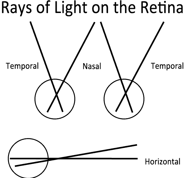
It is important to note that visual field coordinates are the opposite of retinal coordinates. Light entering the eye from the temporal visual field is detected by photoreceptors on the nasal side of the retina and light entering from the nasal visual field is detected by the temporal photoreceptors. Similarly, light from the superior visual field is absorbed in the inferior retina and vice versa. Therefore, a patient with injury to the ganglion cells in the temporal retina would be predicted to have a nasal visual field defect.
Recognition of the visual field extends back more than 2,000 years to the time of Hippocrates, who recognized a hemianopsia [5]. Visual fields are frequently evaluated by simply covering one eye and asking the patient to look straight ahead while using peripheral vision to identify an object, or the number of fingers shown by the examiner. The field is often tested at only four locations, which is sensitive only for large field defects. This method of testing is referred to as confrontation visual field evaluation.
Quantification of visual fields was developed during the nineteenth century. Jannik Bjerrum began mapping visual fields by asking patients to identify whether a white object on the end of a black stick, in front of a black screen, was seen. Several targets of varying sizes on the wand were tested, effectively mapping the variation in size required for vision in different areas of the field. This method of testing, known as the tangent screen, only measures the central 30° of the visual field [5].
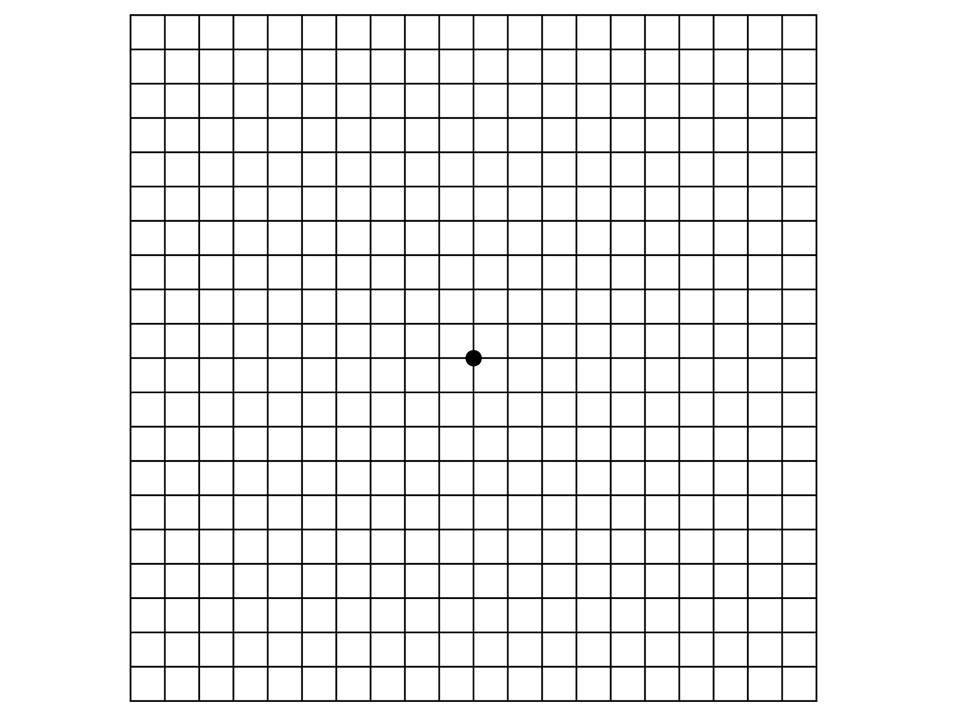
The Amsler grid is another tool for measuring the central visual field occupied by the macula (approximately 8 degrees in diameter). The test consists of a card with horizontal and vertical black lines intersecting on a white background, held at a distance of 25 cm or 40 cm. While fixing gaze on a point in the center of the grid, areas that are blurry, absent, or distorted are identified by the patient. Central vision corresponds with the macula, hence the use of Amsler grids to follow macular pathology clinically [5].
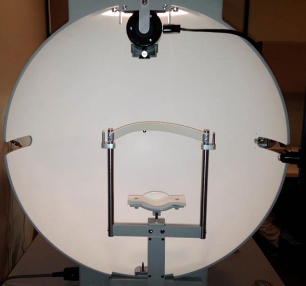
A method of testing the complete visual field was developed by Hans Goldmann. His bowl-shaped perimeter uses bright light as targets superimposed on a white background. Targets may vary in size, luminance, and color. Goldmann perimetry requires trained perimetrists to measure and draw the visual field. Challenges include cost and inter-perimetrist variability [5]. In practice, Goldmann perimetry is a form of kinetic perimetry: a stimulus is moved from beyond the edge of the visual field into the field. The location at which the stimulus is first seen marks the outer perimeter of the visual field for the size of the stimulus tested.
Automated perimetry was developed in the 1970s. As the name suggests, automated perimetry maps a visual field with the aid of a computer. The Octopus perimeter, the Humphrey Field Analyzer, and Humphrey Matrix are a few of the available automated perimeters. Although the Octopus can perform a modified kinetic perimetry, most automated perimetry is static: stationary stimuli, varying in size and intensity, are presented in specific locations within the visual field [6].
Several basic conditions must be met for a successful map of the visual field to be produced by any method. The individual must be able to maintain a constant gaze toward a fixed location for several minutes. Each eye is tested separately while the opposite eye is covered with a patch. Refractive correction must be made with a test lens. Spectacles must not be worn because they can cause false defects in the visual field due to their shape [6]. In addition, correction must be made for presbyopia, to reduce accommodative strain. Standard adjustments for presbyopia are available based on age alone. To correct an astigmatism >0.75 diopters, a cylindrical lens must be used. If the eyelid or lashes obstruct the visual axis, the lid may be taped to the forehead to lift it out of the way.
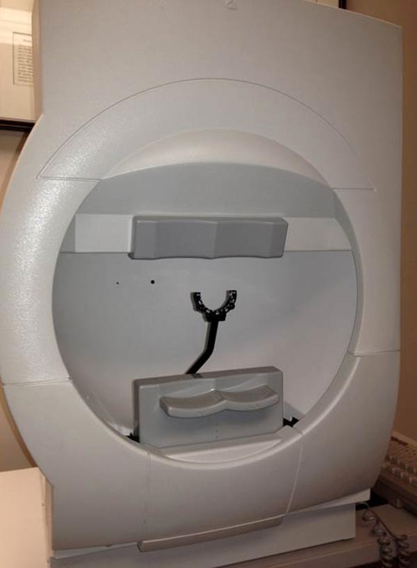
During Humphrey Visual Field (HVF) testing, the patient places his head in the chinrest and fixes his gaze toward a central fixation point in a large, white bowl. As stated above, this test is an example of static perimetry. It assesses the ability to see a non-mobile stimulus which remains for a brief moment (200 ms) in the visual field. When the patient sees a presented stimulus, he presses the button on a handheld remote control. Different locations within a given region of the visual field are tested until the threshold, or the stimulus intensity seen 50% of the time, is seen at each test location.
Stimuli vary in size and luminous intensity. Goldmann size III (about ½ degree in diameter) is generally used, but Goldmann size V (approximately 2 degrees in diameter) is available for patients with decreased visual acuity (< 20/200) or other visual impairment. Goldmann sizes I, II, and III are rarely used clinically. The luminous intensity of the stimuli can be varied over a range of 0.08 to 10,000 apostilbs (asb). It is reported in decibels (dB) of attenuation, or dimming, extending from 0 dB (the brightest, unattenuated stimulus) to 51 dB (the dimmest, maximally attenuated stimulus). If the patient is unable to see even the brightest, unattenuated stimlulus, it is reported as <0 dB.
The Swedish Interactive Thresholding Algorithm (SITA) is frequently used. SITA is a forecasting procedure that uses Bayesian statistical properties that is similar to the methods used for providing weather information and predictions. SITA allows for more rapid analysis than would be possible without forecasting. By taking into account a user's results in nearby locations, stimuli that are unlikely to be seen, or extremely likely to be seen are not tested exhaustively. Instead the stimuli that are likely near threshold are tested.
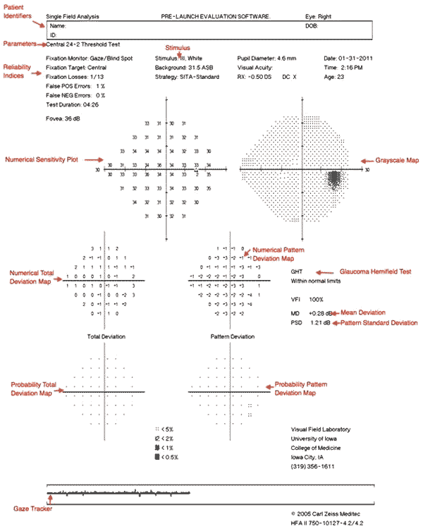
All of the information provided on the visual field printout is important. Patient identity information and the specific test and stimulus size are located near the top of the analysis. It is important to verify that the patient's birthdate was properly entered as an error will result in comparisons with normals in the wrong age group.
Beneath the patient's name is a statement giving information about the testing parameters, such as "Central 24-2 Threshold Test." The first statement, "Central 24" indicates that the central 24 degrees of visual field were analyzed. The next number indicates how the grid of points is aligned to the visual axis. The number "1" indicates that the middle points are overlying the horizontal and vertical meridians. The number "2" indicates that the grid of points straddles these meridians. This is the setting most commonly used, as it is easier to assess whether visual field defects respect the horizontal or vertical midline.
Next on the report are the reliability indices, including fixation losses, false positives, and false negatives. Fixation losses occur when the patient reports seeing a stimulus that is presented in the predicted area of the physiologic blind spot. False positives occur when a patient presses the button when no stimulus is presented. Eager-to-please participants sometimes struggle with high false positive rates (i.e., they are "trigger happy"). False positives can often be corrected by providing a simple statement that many stimuli will not be seen even with normal vision. False negatives occur when a patient fails to see a significantly brighter stimulus at a location than was previously seen. False negatives are usually the result of attention lapses or fatigue and are difficult to correct.
The visual threshold is the intensity of stimulus seen 50% of the time at each location. The threshold values of each tested point are listed in decibels in the sensitivity plot. Higher numbers mean the patient was able to see a more attenuated light, and thus has more sensitive vision at that location. To the right of the numerical sensitivity plot is the grayscale map. This map presents sensitivity across the patient's visual field with lighter regions indicating higher sensitivity and darker regions reflecting lower sensitivity. The sensitivities are not compared to any normative database. Therefore the map may draw attention to an irregularity within a field, but may minimize field loss if loss is more homogenous across the field. Caution should be used as it can be misleading based on where the machine chooses to make the cutoff between the different shades of gray. The raw threshold data should always be assessed in conjunction with the grayscale representation.
The numerical total deviation map compares the patient's visual sensitivity to an average normal individual of the same age. It is useful to compare with age-matched normal thresholds as sensitivity normally decreases gradually with age. Positive values represent areas of the field where the patient can see dimmer stimuli than the average individual of that age. Negative values represent decreased sensitivity from normal.
The numerical pattern deviation map shows discrepancies within a patient's visual field by correcting for generalized decreases in visual sensitivity. It is useful to show localized areas of sensitivity loss hidden within a field that is diffusely depressed. For example, a person with dense cataracts may have decreased threshold across the entire visual field and this may obscure more focal losses due to coexisting disorders like glaucoma. Rather than comparing the patient's threshold values with a normative database, the pattern deviation analysis finds the patient's 7th most sensitive (85th percentile) non-edge point and gives it a value of zero [6]. Each other test location is then compared with this value to correct for any generalized depression. It has been demonstrated that this method is the best for separating widespread or diffuse loss from localized loss.
The bottom-most probability plots are grayscale versions of the total deviation and pattern deviation maps. These maps may be useful to visually represent the statistical significance of the total and pattern deviation calculations. The grayscale maps should only be interpreted in conjunction with the numerical maps to avoid extrapolations.
On the right side of the printout are several useful numbers. The glaucoma hemifield test (GHT) compares groups of corresponding points above and below the horizontal meridian to assess for significant difference which may be consistent with glaucoma. Mean deviation (MD) is the mean deviation in the patient's results compared to those expected from the age-matched normative database. This calculation weighs center points more highly than peripheral points. Pattern standard deviation (PSD) is a depiction of focal defects. It is determined by comparing the differences between adjacent points. Higher values represent more focal losses, while lower values can represent either no loss or diffuse loss. Short-term fluctuations (SF) are a calculation portraying the variability between repeated measurements of the same test location. High SF decreases the reliability of the test. Corrected pattern standard deviation (CPSD) corrects the PSD for the SF. If there is high variability when testing the same point (high SF), PSD is given less weight due to decreased predictive value, and CPSD will therefore appear lower than PSD.
Along the bottom of the HVF printout is a gaze tracker. The patient's pupil is monitored during testing, and each time the pupil moves (representing a loss of fixation or head alignment), an upstroke is recorded. Losses of fixation decrease the accuracy of visual field testing because abnormalities will not correspond with the expected anatomic region of the retina and some may be missed entirely. When the gaze tracker loses view of the pupil (representing a blink or droopy upper eyelid), a downstroke is recorded. Pupillary obstruction can also decrease the accuracy of results.
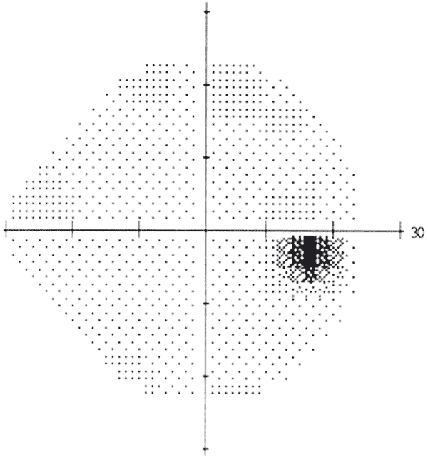
Goldmann visual field (GVF) perimetry is not as widely available as HVF because it requires skilled perimetrists who manually map the visual field without the aid of a computer algorithm. Light is projected into a white bowl with a standardized background light intensity. The projected light forms a fairly circular stimulus. Six stimulus sizes are available, ranging from 0.0625 mm2 (about 6 minutes of arc diameter) to 64 mm2 (about 2 degrees in diameter) when viewed at 30 cm, which is the standard distance between the patient's eye and the stimulus on the background. The overall field mapping technique used is a form of kinetic perimetry, where a stimulus is moved into the field of vision. When the patient sees the stimulus, he indicates so with a low-tech method. At the University of Iowa a washer is given to the patient, with instructions to tap the table with the washer whenever the stimulus is seen. The perimetrist then makes a mark at the point where the stimulus was seen. To account for reaction time, a good perimetrist consistently adjusts the location of the mark. At the conclusion of the tests, the marks are connected by lines to form smooth boundaries of the visual field, or isopters. Areas of decreased sensitivity (scotomata) are mapped by an opposite process, beginning at the center of the area of loss and moving the target outward in at least 8 directions (different clock hours). The different colors used represent stimuli of different sizes and luminous intensities.
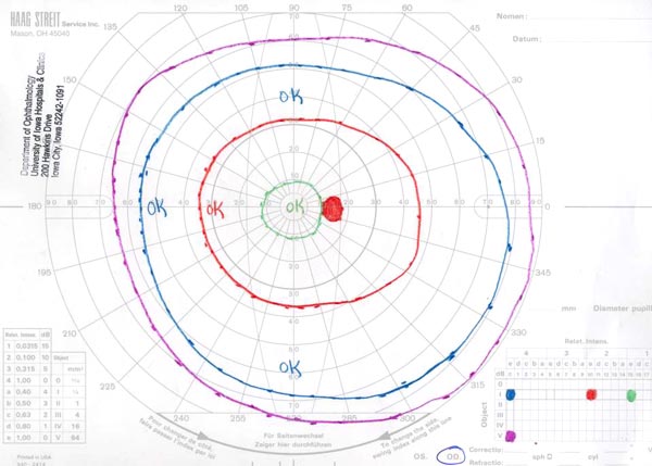
The final result of a GVF is a diagram similar to a topographic map. An analogy commonly used to conceptualize these diagrams is the "island of vision." In this analogy, the visual field is an island with a central peak and the altitude correlates with the visual sensitivity in a given location. In this analogy, physiologic blind spot is represented by a pit or a well in the island. The isopters are named with three characters: a Roman numeral, an Arabic number, and a letter. The Roman numeral indicates the Goldmann size of the stimulus. The Arabic number and letter indicate the attenuation of the light. The combination "4e" is used when there is no attenuation. For each Arabic number less than "4," the light is attenuated by 5 dB. For each letter earlier in the alphabet than "e," the light is attenuated by 1 dB. Within the confines of an isopter, the patient is able to see a light of this size and intensity. Scotomata are represented by areas shaded with a solid color. The color represents the depth of the scotoma, or the dimmest, smallest stimulus the patient is unable to see in that area. For example, in the image below, the physiologic blind spot is shaded orange like the I2e isopter. This suggests the patient is unable to see the I2e stimulus in the area but was able to see the dimmer I4e stimulus.
Loss of optic nerve axons in glaucoma eventually results in visual field defects, but the defects may not be evident until a considerable percentage of axons are lost. After that point in disease progression, further progression can be followed with serial visual field measurements. The visual field defects associated with glaucoma are not specific for the disease. For example, a generalized depression of the entire field is a change associated not only with glaucoma, but could also be the result of a cataract. Additional examples of glaucomatous changes include but are not limited to focal depression, focal or generalized contraction of the visual field, and blind spot baring (reduced sensitivity directly around the optic nerve head) [7].
Scotomata are islands of reduced sensitivity within the visual field surrounded by areas of better vision. Islands shaped like commas are named Seidel scotomata. Islands that arc in the shape of the arcuate fibers are Bjerrum or arcuate scotomata. Those that affect the center of vision are central scotomata and those that are located around the central ten degrees of the visual field are paracentral scotomas. If a defect is located in the nasal field and extends ten degrees along the horizontal meridian in a single isopter, or 5 degrees in multiple isopters, it is known as a nasal step.
End stage glaucoma can result in a superior or inferior hemifield defect, or even loss of all vision other than a central or temporal island of vision. Visual acuity (which is a measure of central vision) may remain 20/20, but the peripheral field of vision may be severely reduced.
Damage to visual mechanisms along various portions of the visual pathways from the optics and photoreceptors up to the visual centers of the brain will produce different shapes and patterns of visual field loss. To assist you in being able to properly interpret visual fields, a table indicating the classic patterns of visual field loss associated with damage to different visual structures is presented, along with a simple "cookbook" for interpreting visual fields is presented at the end of this report. Please keep in mind that the steps of the "cookbook" should be performed in the order specified without shortcuts.
| Patterns Visual Field Loss | Classic Location of Defect |
|---|---|
| Generalized decrease in sensitivity | Media opacity (cornea, lens, or vitreous), decreased attention |
| Constriction of the visual field | Retina, optic nerve, small pupils |
| Ring scotoma | Retina degeneration |
| Central scotoma | Macula or optic nerve |
| Cecocentral scotoma | Papillomacular nerve bundle or nearby retina in region between the macula and optic nerve head |
| Arcuate scotoma | Arcuate retina ganglion cell nerve fiber bundles or retinal vasculature |
| Temporal wedge | Nasal retina radial fibers entering the optic nerve |
| Blind spot enlargement | Optic nerve |
| Multiple scattered defects | Retina |
| Hemifields respecting the horizontal meridian | Retina ganglion cell nerve fiber bundles or less commonly retinal vasculature |
| Hemifields respecting the vertical meridian | Optic chiasm or posterior visual pathways |
| Bitemporal | Optic chiasm |
| Homonymous | Optic chiasm or optic radiations |
| Horizontal tongue | Lateral geniculate body |
| Congruous bilateral defects | Nearer to the posterior visual cortex |
| Incongruous bilateral defects | Nearer to the optic chiasm |
| "Pie in the sky" | Temporal lobe |
| "Pie on the floor" | Parietal lobe |
| "Punched out" defects | Occipital lobe |
Editor's note: The original version switched the classic location of incongruous and congruous defects. Credit to Terry Lu for informing the Editors of this error. Dec. 2021
*These guidelines must be followed in this order for the most accurate results.
Carroll JN, Johnson CA. Visual Field Testing: From One Medical Student to Another. EyeRounds.org. August 21, 2013; available from https://eyerounds.org/tutorials/VF-testing/

Address
University of IowaLegal
Related Links
